Draw Circles on Smooth Sphere Asymptote

6. Applications of Integration

vi.4 Arc Length of a Curve and Surface Area

Learning Objectives

In this section, we use definite integrals to find the arc length of a curve. We tin can think of arc length as the distance you would travel if you were walking forth the path of the curve. Many real-world applications involve arc length. If a rocket is launched along a parabolic path, we might want to know how far the rocket travels. Or, if a bend on a map represents a route, we might want to know how far we accept to bulldoze to reach our destination.

We begin past calculating the arc length of curves defined as functions of $x,$ then nosotros examine the aforementioned process for curves divers every bit functions of $y.$ (The process is identical, with the roles of $x$ and $y$ reversed.) The techniques we employ to find arc length can be extended to notice the surface area of a surface of revolution, and nosotros close the section with an examination of this concept.

Arc Length of the Bend $y$ = $f$ ( $x$ )

In previous applications of integration, nosotros required the role $f(x)$ to be integrable, or at well-nigh continuous. However, for calculating arc length nosotros accept a more stringent requirement for $f(x).$ Here, we require $f(x)$ to be differentiable, and furthermore nosotros require its derivative, ${f}^{\prime }(x),$ to exist continuous. Functions like this, which accept continuous derivatives, are chosen polish . (This property comes upwards again in afterward chapters.)

Let $f(x)$ be a smooth office defined over $\left[a,b\right].$ We want to calculate the length of the curve from the point $(a,f(a))$ to the bespeak $(b,f(b)).$ We showtime past using line segments to approximate the length of the curve. For $i=0,1,2\text{,…},n,$ allow $P=\left\{{x}_{i}\right\}$ be a regular partition of $\left[a,b\right].$ Then, for $i=1,2\text{,…},n,$ construct a line segment from the point $({x}_{i-1},f({x}_{i-1}))$ to the signal $({x}_{i},f({x}_{i})).$ Although it might seem logical to use either horizontal or vertical line segments, we want our line segments to approximate the curve as closely equally possible. (Figure) depicts this construct for $n=5.$

This figure is a graph in the first quadrant. The curve increases and decreases. It is divided into parts at the points a=xsub0, xsub1, xsub2, xsub3, xsub4, and xsub5=b. Also, there are line segments between the points on the curve.

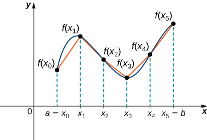
Nosotros tin approximate the length of a curve by adding line segments.

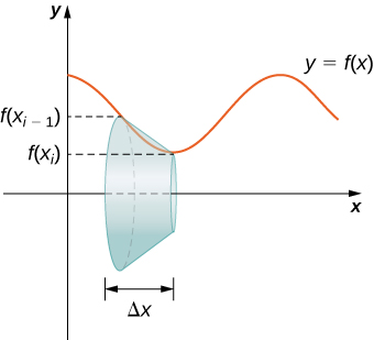
To help u.s.a. discover the length of each line segment, we expect at the change in vertical distance as well every bit the alter in horizontal altitude over each interval. Because we accept used a regular partition, the change in horizontal distance over each interval is given by $\text{Δ}x.$ The modify in vertical distance varies from interval to interval, though, then we use $\text{Δ}{y}_{i}=f({x}_{i})-f({x}_{i-1})$ to correspond the change in vertical altitude over the interval $\left[{x}_{i-1},{x}_{i}\right],$ as shown in (Figure). Annotation that some (or all) $\text{Δ}{y}_{i}$ may be negative.

This figure is a graph. It is a curve above the x-axis beginning at the point f(xsubi-1). The curve ends in the first quadrant at the point f(xsubi). Between the two points on the curve is a line segment. A right triangle is formed with this line segment as the hypotenuse, a horizontal segment with length delta x, and a vertical line segment with length delta y.

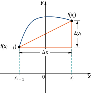
A representative line segment approximates the curve over the interval $\left[{x}_{i-1},{x}_{i}\right].$

Past the Pythagorean theorem, the length of the line segment is $\sqrt{{(\text{Δ}x)}^{2}+{(\text{Δ}{y}_{i})}^{2}}.$ We can also write this as $\text{Δ}x\sqrt{1+{((\text{Δ}{y}_{i})\text{/}(\text{Δ}x))}^{2}}.$ At present, past the Mean Value Theorem, in that location is a bespeak ${x}_{i}^{*}\in \left[{x}_{i-1},{x}_{i}\right]$ such that ${f}^{\prime }({x}_{i}^{*})=(\text{Δ}{y}_{i})\text{/}(\text{Δ}x).$ Then the length of the line segment is given by $\text{Δ}x\sqrt{1+{\left[{f}^{\prime }({x}_{i}^{*})\right]}^{2}}.$ Adding up the lengths of all the line segments, nosotros get

$\text{Arc Length}\approx \underset{i=1}{\overset{n}{\text{∑}}}\sqrt{1+{\left[{f}^{\prime }({x}_{i}^{*})\right]}^{2}}\text{Δ}x.$

This is a Riemann sum. Taking the limit as $n\to \infty ,$ we accept

$\text{Arc Length}=\underset{n\to \infty }{\text{lim}}\underset{i=1}{\overset{n}{\text{∑}}}\sqrt{1+{\left[{f}^{\prime }({x}_{i}^{*})\right]}^{2}}\text{Δ}x={\int }_{a}^{b}\sqrt{1+{\left[{f}^{\prime }(x)\right]}^{2}}dx.$

We summarize these findings in the following theorem.

Annotation that we are integrating an expression involving ${f}^{\prime }(x),$ so we need to be sure ${f}^{\prime }(x)$ is integrable. This is why we require $f(x)$ to be smooth. The following example shows how to apply the theorem.

Calculating the Arc Length of a Role of $x$

Let $f(x)=(4\text{/}3){x}^{3\text{/}2}.$ Calculate the arc length of the graph of $f(x)$ over the interval $\left[0,1\right].$ Round the answer to 3 decimal places.

Solution

$\frac{1}{6}(5\sqrt{5}-1)\approx 1.697$

Although information technology is nice to take a formula for calculating arc length, this particular theorem tin generate expressions that are hard to integrate. We study some techniques for integration in Introduction to Techniques of Integration in the second volume of this text. In some cases, we may have to utilise a computer or calculator to approximate the value of the integral.

Using a Computer or Calculator to Make up one's mind the Arc Length of a Function of $x$

Let $f(x)={x}^{2}.$ Summate the arc length of the graph of $f(x)$ over the interval $\left[1,3\right].$

Solution

We have ${f}^{\prime }(x)=2x,$ then ${\left[{f}^{\prime }(x)\right]}^{2}=4{x}^{2}.$ Then the arc length is given by

$\text{Arc Length}={\int }_{a}^{b}\sqrt{1+{\left[{f}^{\prime }(x)\right]}^{2}}dx={\int }_{1}^{3}\sqrt{1+4{x}^{2}}dx.$

Using a computer to judge the value of this integral, we get

${\int }_{1}^{3}\sqrt{1+4{x}^{2}}dx\approx 8.26815.$

Permit $f(x)= \sin x.$ Calculate the arc length of the graph of $f(x)$ over the interval $\left[0,\pi \right].$ Use a reckoner or calculator to approximate the value of the integral.

Solution

$\text{Arc Length}\approx 3.8202$

Area of a Surface of Revolution

The concepts nosotros used to find the arc length of a curve can be extended to find the surface expanse of a surface of revolution. Surface surface area is the total area of the outer layer of an object. For objects such equally cubes or bricks, the surface area of the object is the sum of the areas of all of its faces. For curved surfaces, the state of affairs is a piddling more than complex. Allow $f(x)$ be a nonnegative smooth function over the interval $\left[a,b\right].$ We wish to find the surface area of the surface of revolution created by revolving the graph of $y=f(x)$ around the $x\text{-axis}$ equally shown in the following effigy.

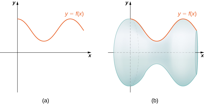
This figure has two graphs. The first graph is labeled

(a) A curve representing the function $f(x).$ (b) The surface of revolution formed by revolving the graph of $f(x)$ around the $x\text{-axis}.$

As we have done many times earlier, we are going to segmentation the interval $\left[a,b\right]$ and approximate the surface expanse by computing the surface surface area of simpler shapes. Nosotros start by using line segments to gauge the bend, as we did earlier in this department. For $i=0,1,2\text{,…},n,$ let $P=\left\{{x}_{i}\right\}$ exist a regular segmentation of $\left[a,b\right].$ And so, for $i=1,2\text{,…},n,$ construct a line segment from the indicate $({x}_{i-1},f({x}_{i-1}))$ to the point $({x}_{i},f({x}_{i})).$ At present, revolve these line segments around the $x\text{-axis}$ to generate an approximation of the surface of revolution as shown in the following figure.

This figure has two graphs. The first graph is labeled

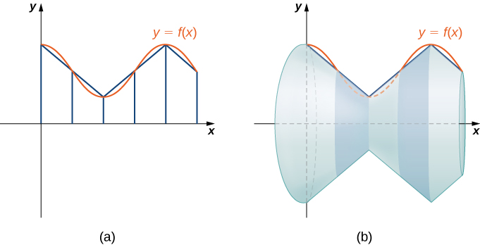
(a) Approximating $f(x)$ with line segments. (b) The surface of revolution formed by revolving the line segments effectually the $x\text{-axis}.$

Discover that when each line segment is revolved effectually the centrality, it produces a band. These bands are actually pieces of cones (retrieve of an ice cream cone with the pointy end cut off). A piece of a cone similar this is called a frustum of a cone.

To notice the surface expanse of the band, nosotros need to notice the lateral surface area, $S,$ of the frustum (the area of just the slanted outside surface of the frustum, not including the areas of the top or lesser faces). Let ${r}_{1}$ and ${r}_{2}$ be the radii of the wide end and the narrow end of the frustum, respectively, and let $l$ be the slant height of the frustum as shown in the following effigy.

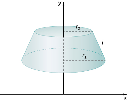
This figure is a graph. It is a frustum of a cone above the x-axis with the y-axis in the center. The radius of the bottom of the frustum is rsub1 and the radius of the top is rsub2. The length of the side is labeled

A frustum of a cone tin approximate a pocket-size part of surface expanse.

We know the lateral surface area of a cone is given past

$\text{Lateral Surface Area}=\pi rs,$

where $r$ is the radius of the base of operations of the cone and $s$ is the slant height (see the following figure).

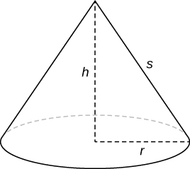
This figure is a cone. The cone has radius r, height h, and length of side s.

The lateral surface area of the cone is given past $\pi rs.$

Since a frustum can be thought of as a piece of a cone, the lateral surface area of the frustum is given by the lateral area of the whole cone less the lateral expanse of the smaller cone (the pointy tip) that was cut off (see the post-obit figure).

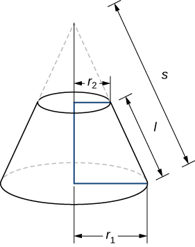
This figure is a graph. It is a frustum of a cone. The radius of the bottom of the frustum is rsub1 and the radius of the top is rsub2. The length of the side is labeled

Calculating the lateral surface area of a frustum of a cone.

The cross-sections of the pocket-size cone and the large cone are similar triangles, then we see that

$\frac{{r}_{2}}{{r}_{1}}=\frac{s-l}{s}.$

Solving for $s,$ we get

$\begin{array}{ccc}\hfill \frac{{r}_{2}}{{r}_{1}}& =\hfill & \frac{s-l}{s}\hfill \\ \hfill {r}_{2}s& =\hfill & {r}_{1}(s-l)\hfill \\ \hfill {r}_{2}s& =\hfill & {r}_{1}s-{r}_{1}l\hfill \\ \hfill {r}_{1}l& =\hfill & {r}_{1}s-{r}_{2}s\hfill \\ \hfill {r}_{1}l& =\hfill & ({r}_{1}-{r}_{2})s\hfill \\ \hfill \frac{{r}_{1}l}{{r}_{1}-{r}_{2}}& =\hfill & s.\hfill \end{array}$

Then the lateral surface surface area (SA) of the frustum is

$\begin{array}{cc}\hfill S& =\text{(Lateral SA of large cone)}-\text{(Lateral SA of small cone)}\hfill \\ & =\pi {r}_{1}s-\pi {r}_{2}(s-l)\hfill \\ & =\pi {r}_{1}(\frac{{r}_{1}l}{{r}_{1}-{r}_{2}})-\pi {r}_{2}(\frac{{r}_{1}l}{{r}_{1}-{r}_{2}}-l)\hfill \\ & =\frac{\pi {r}_{1}^{2}l}{{r}_{1}-{r}_{2}}-\frac{\pi {r}_{1}{r}_{2}l}{{r}_{1}-{r}_{2}}+\pi {r}_{2}l\hfill \\ & =\frac{\pi {r}_{1}^{2}l}{{r}_{1}-{r}_{2}}-\frac{\pi {r}_{1}{r}_{2}l}{{r}_{1}-{r}_{2}}+\frac{\pi {r}_{2}l({r}_{1}-{r}_{2})}{{r}_{1}-{r}_{2}}\hfill \\ & =\frac{\pi {r}_{1}^{2}l}{{r}_{1}-{r}_{2}}-\frac{\pi {r}_{1}{r}_{2}l}{{r}_{1}-{r}_{2}}+\frac{\pi {r}_{1}{r}_{2}l}{{r}_{1}-{r}_{2}}-\frac{\pi {r}_{2}{}^{2}l}{{r}_{1}-{r}_{2}}\hfill \\ & =\frac{\pi ({r}_{1}^{2}-{r}_{2}^{2})l}{{r}_{1}-{r}_{2}}=\frac{\pi ({r}_{1}-{r}_{2})({r}_{1}+{r}_{2})l}{{r}_{1}-{r}_{2}}=\pi ({r}_{1}+{r}_{2})l.\hfill \end{array}$

Allow'due south at present utilise this formula to calculate the surface surface area of each of the bands formed past revolving the line segments around the $x\text{-axis}\text{.}$ A representative band is shown in the post-obit figure.

This figure has two graphics. The first is a curve in the first quadrant. Around the x-axis is a frustum of a cone. The edge of the frustum is against the curve. The edge begins at f(xsubi-1) and ends at f(xsubi). The second image is the same curve with the same frustum. the height of the frustum is delta x and the curve is labeled y=f(x).

A representative band used for determining surface area.

Note that the slant height of this frustum is just the length of the line segment used to generate information technology. And then, applying the surface area formula, nosotros take

$\begin{array}{cc}\hfill S& =\pi ({r}_{1}+{r}_{2})l\hfill \\ & =\pi (f({x}_{i-1})+f({x}_{i}))\sqrt{\text{Δ}{x}^{2}+{(\text{Δ}{y}_{i})}^{2}}\hfill \\ & =\pi (f({x}_{i-1})+f({x}_{i}))\text{Δ}x\sqrt{1+{(\frac{\text{Δ}{y}_{i}}{\text{Δ}x})}^{2}}.\hfill \end{array}$

Now, every bit we did in the development of the arc length formula, we apply the Hateful Value Theorem to select ${x}_{i}^{*}\in \left[{x}_{i-1},{x}_{i}\right]$ such that ${f}^{\prime }({x}_{i}^{*})=(\text{Δ}{y}_{i})\text{/}\text{Δ}x.$ This gives usa

$S=\pi (f({x}_{i-1})+f({x}_{i}))\text{Δ}x\sqrt{1+{({f}^{\prime }({x}_{i}^{*}))}^{2}}.$

Furthermore, since $f(x)$ is continuous, by the Intermediate Value Theorem, there is a point ${x}_{i}^{**}\in \left[{x}_{i-1},{x}_{i}\right]$ such that $f({x}_{i}^{**})=(1\text{/}2)\left[f({x}_{i-1})+f({x}_{i})\right],$ so nosotros go

$S=2\pi f({x}_{i}^{**})\text{Δ}x\sqrt{1+{({f}^{\prime }({x}_{i}^{*}))}^{2}}.$

And so the approximate expanse of the whole surface of revolution is given by

$\text{Surface Area}\approx \underset{i=1}{\overset{n}{\text{∑}}}2\pi f({x}_{i}^{**})\text{Δ}x\sqrt{1+{({f}^{\prime }({x}_{i}^{*}))}^{2}}.$

This almost looks like a Riemann sum, except we have functions evaluated at two different points, ${x}_{i}^{*}$ and ${x}_{i}^{**},$ over the interval $\left[{x}_{i-1},{x}_{i}\right].$ Although nosotros practice non examine the details here, it turns out that considering $f(x)$ is smooth, if we allow $n\to \infty ,$ the limit works the same as a Riemann sum fifty-fifty with the two different evaluation points. This makes sense intuitively. Both ${x}_{i}^{*}$ and ${x}_{i}^{**}$ are in the interval $\left[{x}_{i-1},{x}_{i}\right],$ so it makes sense that as $n\to \infty ,$ both ${x}_{i}^{*}$ and ${x}_{i}^{**}$ approach $x.$ Those of y'all who are interested in the details should consult an advanced calculus text.

Taking the limit as $n\to \infty ,$ nosotros become

$\text{Surface Area}=\underset{n\to \infty }{\text{lim}}\underset{i=1}{\overset{n}{\text{∑}}}2\pi f({x}_{i}^{**})\text{Δ}x\sqrt{1+{({f}^{\prime }({x}_{i}^{*}))}^{2}}={\int }_{a}^{b}(2\pi f(x)\sqrt{1+{({f}^{\prime }(x))}^{2}})dx.$

As with arc length, we can conduct a similar development for functions of $y$ to get a formula for the surface area of surfaces of revolution most the $y\text{-axis}.$ These findings are summarized in the following theorem.

Computing the Surface area of a Surface of Revolution 1

Computing the Surface area of a Surface of Revolution 2

Fundamental Concepts

The arc length of a curve tin can be calculated using a definite integral.
The arc length is first approximated using line segments, which generates a Riemann sum. Taking a limit then gives usa the definite integral formula. The aforementioned process tin can be applied to functions of $y.$
The concepts used to calculate the arc length can be generalized to observe the surface surface area of a surface of revolution.
The integrals generated by both the arc length and surface area formulas are often difficult to evaluate. Information technology may be necessary to employ a computer or calculator to estimate the values of the integrals.

Key Equations

For the post-obit exercises, find the length of the functions over the given interval.

1. $y=5x\text{from}x=0\text{ to }x=2$

Solution

$2\sqrt{26}$

ii. $y=-\frac{1}{2}x+25\text{from}x=1\text{ to }x=4$

3. $x=4y\text{from}y=-1\text{ to }y=1$

Solution

$2\sqrt{17}$

4.Selection an arbitrary linear role $x=g(y)$ over whatever interval of your pick $({y}_{1},{y}_{2}).$ Decide the length of the function and then testify the length is correct by using geometry.

Solution

$\frac{\pi }{6}(17\sqrt{17}-5\sqrt{5})$

For the post-obit exercises, detect the lengths of the functions of $x$ over the given interval. If y'all cannot evaluate the integral exactly, use technology to approximate it.

eight. $y={x}^{2\text{/}3}$ from $(1,1)\text{ to }(8,4)$

12. $y=\frac{{x}^{3}}{3}+\frac{1}{4x}$ from $x=1\text{ to }x=3$

14. $y=\frac{2{x}^{3\text{/}2}}{3}-\frac{{x}^{1\text{/}2}}{2}$ from $x=1\text{ to }x=4$

15. $y=\frac{1}{27}{(9{x}^{2}+6)}^{3\text{/}2}$ from $x=0\text{ to }x=2$

sixteen. [T] $y= \sin x$ on $x=0\text{ to }x=\pi$

For the following exercises, find the lengths of the functions of $y$ over the given interval. If you cannot evaluate the integral exactly, use technology to judge it.

18. $x=\frac{1}{2}({e}^{y}+{e}^{\text{−}y})$ from $y=-1\text{ to }y=1$

25. [T] $x={4}^{y}$ from $y=0\text{ to }y=2$

For the following exercises, discover the surface area of the volume generated when the post-obit curves revolve around the $x\text{-axis}.$ If you cannot evaluate the integral exactly, use your computer to gauge it.

xxx. [T] $y=\frac{1}{{x}^{2}}$ from $x=1\text{ to }x=3$

32. $y=\sqrt{4-{x}^{2}}$ from $x=-1\text{ to }x=1$

34. [T] $y= \tan x$ from $x=-\frac{\pi }{4}\text{ to }x=\frac{\pi }{4}$

For the following exercises, observe the surface area of the volume generated when the post-obit curves revolve effectually the $y\text{-axis}\text{.}$ If yous cannot evaluate the integral exactly, use your calculator to approximate it.

36. $y=\frac{1}{2}{x}^{2}+\frac{1}{2}$ from $x=0\text{ to }x=1$

Solution

$2\pi$

47. [T] You are building a bridge that will span 10 ft. You intend to add decorative rope in the shape of $y=5| \sin ((x\pi )\text{/}5)|,$ where $x$ is the distance in feet from ane stop of the span. Find out how much rope you need to buy, rounded to the nearest foot.

For the post-obit exercises, notice the exact arc length for the following issues over the given interval.

54.Explicate why the surface area is space when $y=1\text{/}x$ is rotated around the $x\text{-axis}$ for $1\le x<\infty ,$ merely the book is finite.

Solution

For more information, look upwardly Gabriel's Horn.

Glossary

arc length: the arc length of a curve can be thought of every bit the distance a person would travel along the path of the curve

frustum: a portion of a cone; a frustum is synthetic by cut the cone with a plane parallel to the base

surface area: the surface surface area of a solid is the full area of the outer layer of the object; for objects such equally cubes or bricks, the surface area of the object is the sum of the areas of all of its faces

bratcheryousbantor.blogspot.com

Source: https://opentextbc.ca/calculusv1openstax/chapter/arc-length-of-a-curve-and-surface-area/

Draw Circles on Smooth Sphere Asymptote

vi.4 Arc Length of a Curve and Surface Area

Learning Objectives

Arc Length of the Bend $y$ = $f$ ( $x$ )

Calculating the Arc Length of a Role of $x$

Solution

Using a Computer or Calculator to Make up one's mind the Arc Length of a Function of $x$

Solution

Solution

Area of a Surface of Revolution

Computing the Surface area of a Surface of Revolution 1

Computing the Surface area of a Surface of Revolution 2

Fundamental Concepts

Key Equations

Solution

Solution

Solution

Solution

Solution

Glossary

0 Response to "Draw Circles on Smooth Sphere Asymptote"

Post a Comment

Iklan Atas Artikel

Iklan Tengah Artikel 1

Iklan Tengah Artikel 2

Iklan Bawah Artikel

Draw Circles on Smooth Sphere Asymptote

vi.4 Arc Length of a Curve and Surface Area

Learning Objectives

Arc Length of the Bend = ()

Calculating the Arc Length of a Role of

Solution

Using a Computer or Calculator to Make up one's mind the Arc Length of a Function of

Solution

Solution

Area of a Surface of Revolution

Computing the Surface area of a Surface of Revolution 1

Computing the Surface area of a Surface of Revolution 2

Fundamental Concepts

Key Equations

Solution

Solution

Solution

Solution

Solution

Glossary

0 Response to "Draw Circles on Smooth Sphere Asymptote"

Post a Comment

Iklan Atas Artikel

Iklan Tengah Artikel 1

Iklan Tengah Artikel 2

Iklan Bawah Artikel

Arc Length of the Bend $y$ = $f$ ( $x$ )

Calculating the Arc Length of a Role of $x$

Using a Computer or Calculator to Make up one's mind the Arc Length of a Function of $x$